RainGAN — Synthesized Environmental Audio
Just as some like to listen to white noise, I like listening to rain to relax and focus. When I’m studying, I love to put on my earbuds and stream those 24-hr livestreams of nothing but rain sounds. One day I thought, what if we could create procedurally generated rain sounds with ML?
300 hours of training later on 1 Colab GPU, these are the results (volume warning):
The neural network behind these results was trained on data that sounds like this:
The preceding video was transformed into a .wav file and clipped from 0:0:01 to 0:6:30.
Motivations — Why Rain?
Applying generative neural networks to audio data is not entirely novel. But even at the cutting edge of deep learning today, there are challenges with training neural networks to understand highly structured audio sequences, like pop songs. Strategies like LSTMs, attention, and transformers are a continuing area of study for how to better represent long-term dependencies within audio data. At the cutting edge are algorithms like Jukebox by OpenAI are famed for recreating songs in the style of different artists.
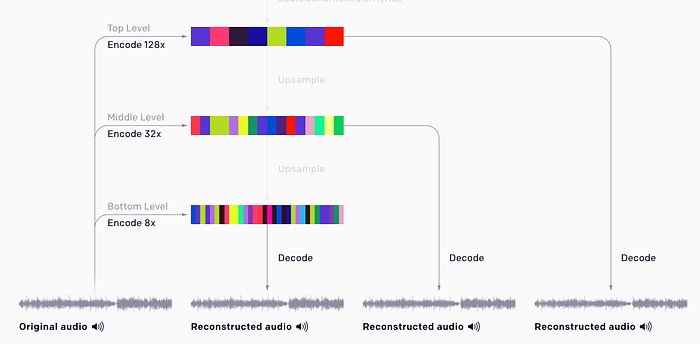
Looking at the literature, one would quickly find that current AI’s struggle to understand the structures within song music. Listening to Jukebox’s handpicked results, one could quickly hear that the algorithm struggles to *end* a song; the results feel like a never-ending run-on sentence. These networks also struggle to self-learn the characteristic bar structures (verse, chorus, etc.) in song music. TL:DR song music is tough to generate convincingly.
Rain sounds have the advantage over other types of audio data due to its pseudo-randomness. There aren’t discernable patterns, and each second of sound feels loosely related to the next.
The Strategy
The training audio was recorded at a 48k sampling frequency. That means one second of audio contains 48,000 data points! (Times two, if you’re considering both left and right sound channels!) Needless to say, training off of an input size this massive is incredibly memory intensive and slow.
So how can we process audio data to make it more trainable?
One tactic is to train on batches of 0.5s samples. Because of the randomness of rain, these batches can even be shuffled for even more stable training.
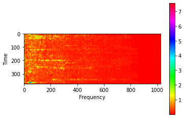
Then, these audio samples can be converted into a 2D “spectrogram” image. Spectrograms display the frequencies over time in the audio data. This can be done with the TensorFlow IO module tfio.audio.spectrogram.
tfio.audio.spectrogram(
    input, nfft, window, stride, name=None
)
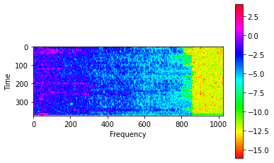
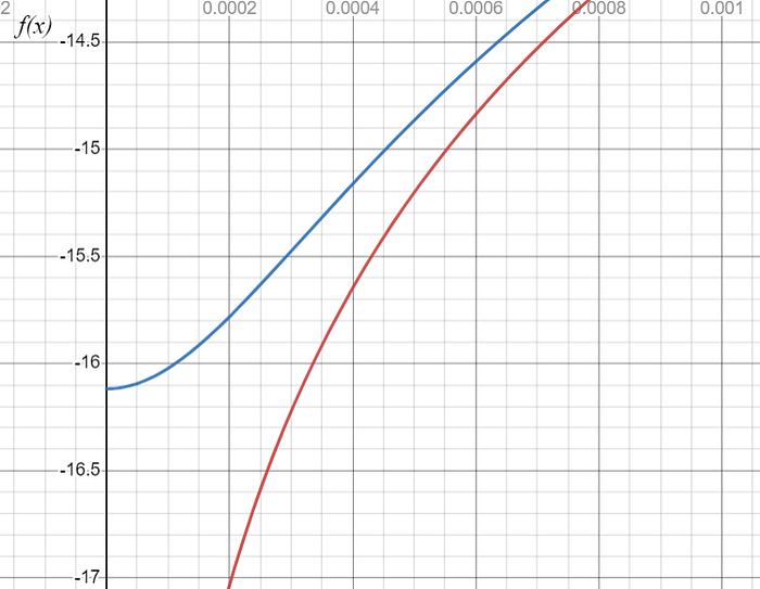
This article describes a quick way to further enhance the base spectrogram image for more trainable features. This process involves taking the log of the square of the spectrogram values. My implementation includes a small scalar offset to prevent errors arising from negative infinity values.
real_image = tfio.audio.spectrogram(audio_batch[0], nfft=2048, window=1024, stride=64)noise = tf.random.truncated_normal([1, noise_dim])generated_image = model.generator(noise, training=False)[0]modified_image = tf.math.log(tf.math.pow(real_image,2)+0.0000001)max = tf.reduce_max(modified_image)min = tf.reduce_min(modified_image)generated_image = generated_image * (max - min) + mingenerated_image = tf.math.sqrt(tf.math.exp(generated_image))
The difference this offset makes is illustrated here:
After these steps, the image size for 0.5s of data is still 375x1025. In experimentation, down sampling with bicubic interpolation and up sampling with area interpolation did well to preserve detail while shrinking input size. These sampling methods were chosen per the recommendations in this article: OpenCV — comparison of interpolation algorithms when resizing an image — Opencvpython. Resizing to and from a square image of 256x256 was found to be ideal for this project. (The fact that the aspect ratio is not preserved and that the image is squashed may actually assist training in this case. It may help the network more easily generate the specific shapes common in the training data.)
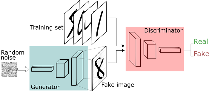
The GAN’s generator may then output an image also in 256x256 size. The discriminator is trained to discern real and fake augmented spectrograms of 256x256 size. The generated fake image can then be up-sampled to 375x1025. Then a TensorFlow IO’s inverse spectrogram function can be applied to get the resulting synthesized audio.
tfio.audio.inverse_spectrogram(
    spectrogram, nfft, window, stride, iterations=30
)
To learn more about setting up a basic DCGAN (Deep Convolutional GAN) follow TensorFlow’s tutorial here.
Upgrading the GAN
There are several strategies to further improve training efficiency and results of the DCGAN for this project. There are several known issues with GANs, like in regard to the stability of training.
The cutting edge of GANs are BigGANs which set forth some guidelines we can follow to improve our model performance. (Note that state-of-the-art BigGANs connected with image synthesis are trained on a prohibitively high number of GPUs available to large institutions, while this project is designed to be run on 1 GPU.)

Large Latent Space
The generator builds spectrogram images from a random 256-dimensional vector. A larger latent space enables the model to learn more nuanced descriptions of data, at the cost of training speed.
Spectral Normalization
Spectral normalization layers precede batch normalization layers in the generator.
Spectral Normalization for Generative Adversarial Networks, 2018
Kernels and Activations
Small kernel sizes are used in both generator and discriminator. Research suggest that more layers of smaller kernels can outperform fewer layers with larger kernels.
LeakyRELU is used for the discriminator, RELU is used for the generator.
Loss Functions
Are Gans Created Equal? A Large-Scale Study, 2017 suggests that there is a negligible difference in performance of different loss functions for GANs. Some common loss functions used for a deep GAN are hinge loss and Wasserstein loss.
For this project, the vanilla NS GAN loss provided in TensorFlow’s DCGAN tutorial is used.
Self-Attention Layers
Self-attention layers are embedded into the generator model. Self-attention in SAGANs have been shown to improve a model’s understanding of structural relations in an image. For example, in conventional image synthesis, self-attention enables a GAN to understand that an image of a dog is more than a blob and that it should include four legs.
Truncation Trick
Generated images are sampled from a truncated normal distribution. This has shown to help improve quality of generated results at the cost of some variety. For this project, values outside of 3 stdevs are resampled.
Reflections
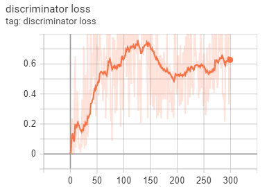
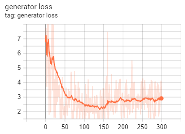
The results of the training accurately capture the general shape of rain audio. Sounds of individual “loud” droplets can be discerned. However, the model struggles to reproduce the smaller, more cacophonous droplet sounds realistically. There sounds like artifacts at specific high frequencies. Interestingly, when played on a speaker as opposed to headphones, the rain sounds more realistic.
Future Improvements
- Mel Spectrogram: converting to a mel spectrogram would have the purpose of better differentiating frequencies that humans are better at distinguishing. Using different forms of spectrogram manipulation may yield more human-friendly results.
- Concatenated Discriminator: one idea is to input multiple spectrograms of different parameters into the discriminator. The concept is to target different frequency ranges with separate spectrograms to raise the ceiling on discriminator performance.
- Log shift: a scalar shift of 0.0000001 is added to spectrogram values before a log operation is performed. This truncates the lower bound of data to -7. Reducing the magnitude of this shift could improve fidelity of lower intensity frequencies.
- WGAN and hinge loss: different loss functions may more quickly converge on a solution. It could be useful to experiment with other common GAN losses.
Further Reading
- A Gentle Introduction to BigGAN the Big Generative Adversarial Network (machinelearningmastery.com)
- How to Implement Wasserstein Loss for Generative Adversarial Networks (machinelearningmastery.com)
- Do GAN Loss Functions Really Matter? | DeepAI
- Audio Deep Learning Made Simple (Part 2): Why Mel Spectrograms perform better | by Ketan Doshi | Towards Data Science
